In a Nutshell:

• Policy analysis can be enhanced by identifying a subset of peer states to use as a basis of comparison. It is important to adopt an approach thoughtfully, as these comparison states may influence subsequent findings.
• Our method of identifying peer states uses simple, effective, and transparent metrics related to population, the road system, land use, and the local climate and geology. The approach could be adapted to use any available state-specific data.
• We conclude that Michigan’s top four peer states for evaluating transportation infrastructure policy are Ohio, Indiana, Virginia, and Georgia. Second-tier peer states were also identified. These findings will be useful in future analyses of Michigan’s transportation funding levels, policies, and outcomes.

By Eric Paul Dennis, PE. epdennis@CRCMich.org

The Task: Identifying Michigan’s ‘Peer States’ for Policy Analysis

In public policy analysis, it is difficult to identify any specific approach as a best practice. While we are driven by several policy goals (e.g., efficiency, accountability, equity) it helps to know what ‘success’ looks like by comparing our state, cities, school districts, etc. to similar governments. To leverage various approaches by state and local governments as ‘laboratories of democracy,’ it is necessary to measure and compare the outcomes of policies.

In a series of articles to be published in 2024, we will compare Michigan’s transportation infrastructure to other states in an effort to identify our strengths, weaknesses, opportunities, and threats. However, with 50 states, all unique in their own way, it can be more useful to select a specific subset of peer states to use as a basis of comparison. With this in mind, the Citizens Research Council has constructed a transportation infrastructure peer state index to determine which U.S. states are most similar to Michigan for purposes of examining infrastructure policy and planning (map below).

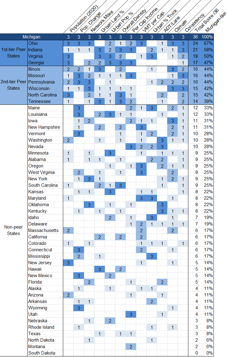
Image: States with Transportation Infrastructure Systems Similar to Michigan.

The Component Metrics

Any approach to selecting peer states requires informed creativity. Numerous statistics might be important and there are practically infinite ways of combining them into a final result. Our approach uses data from the Federal Highway Administration’s 2020 Highway Statistics Series combined with additional census data and research findings. These metrics are most pertinent to transportation infrastructure policy but many are relevant to other infrastructure types as well.

For each of 12 individual categories, raw data was rank-ordered as most similar to Michigan and scored with up to three ‘similarity points.’ Unless stated otherwise, the five closest states are awarded 3 points each, the next five are awarded 2 points, and the next ten are awarded one point. The final index is the sum of points awarded across all categories expressed as a percentage of all possible points (36).

The 12 individual components are:

1. Population (2020 Census)

The 2020 statewide population provides a rough idea of the demands placed on public infrastructure and resources available. Michigan is the tenth largest state with a population of just over ten million people. The mean U.S. state population is about 6.2 million, and the median is only 4.4 million.

2. Population Change (2010-2020)

Infrastructure issues and related policy can vary depending on if a state is growing and how fast. Michigan grew 2.0 percent from 2010 to 2020, one of nine states to see population growth between zero and 3 percent. When scoring this category, these states were given 3 similarity points. Three states – West Virginia, Mississippi, and Illinois – lost population and were scored 2 points each. Michigan’s situation is not too dissimilar from these shrinking states, as Michigan did experience net loss in the preceding decade and is projected to have roughly flat population growth for the foreseeable future. Additionally, ten states grew between 3 percent  and 5 percent, not too dissimilar from Michigan’s 2 percent growth; these were scored 1 point. (Note: The other metrics that embed population statistics use 2010 Census data because the FHWA dataset has not yet been updated with 2020 data.)

3. Network Miles (public road centerline length)

The geographical size of a state factors into the demands placed on road agencies to provide access to sparsely populated rural areas. However, many large states are so sparsely populated that the public road network has gaps of tens or hundreds of miles. Alaska is the best example of this–while it is the largest state by land area, it ranks 45th in miles of public road. Rather than using the area of a state as a basis for comparison, it is more relevant to consider the size of the public road network in centerline miles, which reflects the size of the state but more directly defines the demands placed on road agencies. Michigan is the 22nd largest state in land area, but has the 10th most extensive public road network with 256,295 reported miles of public road.

4. Urban Land Area Percentage

The percentage of a state’s land area that is defined as “urban” helps define the demands placed on infrastructure and the efficiency with which infrastructure can be constructed and maintained. States with similar urban land percentages share similar priorities and constraints in allocating resources between urban and rural areas. Michigan is the 15th most urbanized state by land area with 6.4 percent of its area designated as urban. This is below the U.S. mean of 7.4 percent but above the median state, which has only 3.5 percent urban area.

5. Urban Population Percentage

The percentage of a state’s population living in urban areas does not always correlate closely with percent urban by land area. For example, California is the nation’s most urbanized state with a population that is 95 percent urban, yet California is the 21st most urbanized state by land area with 5.3 percent, a slightly lesser percentage than Michigan. States with higher percentages of urban population are often better positioned to provide infrastructure efficiently. Michigan’s urban population is 24th at 74.6 percent, very near the median state with 73.7 percent and the U.S. mean of 73.6 percent urbanized.

6. Overall Density of Polulation

A third way of quantifying population distribution within a state is overall density (i.e., in residents per square mile). By this measure, Michigan is the 17th densest state with 175 persons per square mile. Michigan is less dense than the U.S. average of 195, but more dense  than the median state of 99 persons per square mile. Combined with the above metrics reflecting urban area and population, this metric can identify states with similar overall land use to Michigan.

7. Per Capita Income

Per capita income is a useful way to broadly reflect a state’s economic activity and potential funding resources, as well as vehicle trips generated by economic activity. Michigan’s per capita income of $51,971 ranks 34th. This is below both the U.S. average of $56,868 and the median state of $55,403. (Reflects data provided by FHWA Table PS-1 for year 2020.)

8. VMT per Capita

Annual vehicle miles traveled (VMT) per capita is simply the estimated total annual VMT in a state divided by the number of residents. Michigan ranked 37th for most VMT per capita, indicating the state has relatively less traffic than the U.S. average of 10,054 VMT/cap and the median state of 8,909 VMT/cap. The states with high VMT per capita tend to be states with a low percentage urban population and/or that are situated along high-traffic interstate routes.

9. Urban Percentage Truck VMT

Truck traffic imposes a disproportionate amount of the damage on road pavement. Cars and light trucks impose demands on the road system that can lead to congestion and safety issues, but have negligible impact on roadway pavement. Thus, the percentage of VMT associated with trucks and heavy vehicles correlates closely with the costs of providing appropriate roadway pavement and maintaining it in good condition. Urban areas with heavy truck traffic also have unique issues related to congestion, safety, and traffic control. Typically, states with high VMT and a high percentage of trucks may require substantial resources to accommodate such demands. Fortunately, not only is Michigan a low VMT per capita state, but it is a very low truck traffic state. Michigan ranks 46th among states with an urban percentage truck VMT of 5.6 percent. In other words, only four states have fewer truck miles as a percentage of urban traffic.

10. Average Daily Traffic (ADT) per lane (all arterials)

Average daily traffic per lane across the state broadly reflects traffic density, which then reflects the likelihood of congestion. This metric is influenced both by traffic demand (ADT) and capacity to accommodate that demand (number of lanes). States that are similar in this regard are likely to have similar concerns regarding traffic management, congestion mitigation, and capacity constraints. Michigan ranks 22nd for highest trafficked arterial lanes with 6,027 vehicles per lane per day. This is slightly higher than the U.S. state average of 5,571 and the median state 5,764.

11. Climate

Although heavy trucks do the most damage to roadway pavement, the local climate can also significantly factor into pavement failure. For example, pavement can be rapidly damaged during freeze/thaw cycles, especially in regions where soils are likely to be saturated in the spring. Climate also has implications for the design, maintenance, and operations of water and energy infrastructure. 

A study by Michigan Technological University (MTU) found that Michigan’s climate was closest to Iowa, Wisconsin, Illinois, and Ohio. Michigan and these four states are all within the wet-freeze climate zone as defined by FHWA, experiencing seasonal freeze/thaw cycling and saturated soils. Another way of estimating freeze-thaw activity is the Lienhart freeze-thaw index, which combines seasonal temperature and precipitation into a single metric. As shown below, Michigan’s average Leinhart freeze-thaw index is about 40. This is towards the higher end of the range but not dissimilar from many areas in the U.S. northeast and northwest. 

Image: Isoline map of the Lienhart moist freeze-thaw index shows that Michigan is part of a region challenged by freeze-thaw cycling.

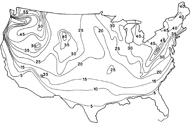
Source: Lienhart. (1988.)

In scoring the climate factor, 3 points were awarded to the four states identified by MTU as most climatically similar to Michigan. Two (2) points were awarded to all other states within the FHWA wet-freeze region that also have a similar Lienhart freeze-thaw index as Michigan. One (1) point was awarded to the remainder of the states within the FHWA wet-freeze region. Finally, 1 point was also awarded to states in the FHWA dry-freeze region that have a similar Leinhart freeze-thaw index as Michigan.

12. Consistency Bonus

The final metric reflects the number of previous categories in which states matched up with Michigan. This was done because states that are consistently grouped with Michigan are more likely to have similar infrastructure issues than states that match fewer categories more closely. This consistency bonus amplifies the results of previous categories, helping to make the most appropriate peer states more obvious. States that matched in eight or more of the eleven categories (IN, MO, OH, and WI) were awarded an additional 3 points. States matching seven categories were awarded 2 points. Finally, 1 consistency point was given to states matching five or six categories.

Results: Michigan’s Infrastructure Peer States

The table below shows that full scoring that determined Michigan’s infrastructure peer states. The results are further divided into first- and second-tier peer states.  

Table: Full scoring of Michigan’s Infrastructure Peers States

First-tier Peer States

After final scoring, four states emerged as distinctly similar to Michigan: Ohio, Indiana, Virginia, and Georgia.

The top two peer states, Ohio and Indiana, are no surprise. Each share a border with Michigan, as well as Great Lakes coastline, and have similar socioeconomics resulting from historic economic bases in manufacturing and heavy industry.

Ohio is similar to Michigan in all but two categories. One difference is urban percentage by land area. Ohio is significantly more urban by percentage land area, though it is similar along other land-use metrics. Additionally, Ohio’s urban traffic is more heavily weighted towards trucks–likely a result of interstate freight corridors. 

Indiana scored points on all but one category, VMT per capita, where it is much higher than Michigan. While Indianapolis has laudable urban form, Indiana is otherwise a notably suburban sprawly state, contributing to its high VMT per capita. Also contributing to VMT, Indiana carries substantial freight traffic and has become something of a freight industry hub. However Indiana’s freight traffic is largely pass-through along rural interstates, and so the impact of this truck traffic on urban areas is on the lower end of the spectrum (along with Michigan). 

Virginia and Georgia may not be obvious choices as peer states for Michigan, but a review of the data confirms the results. In terms of population distribution, land use, and economic activity, Virginia and Georgia are very similar to Michigan. The main difference is the direction from which they’ve reached their current configuration. Michigan, Ohio, and Indiana were once more populous, wealthier states, but have experienced stagnant growth in recent decades. Georgia and Virginia were once very rural, agricultural states, but have experienced rapid growth in recent decades. In future decades, these states may diverge. But our data shows that at this point in time, these states are very similar.

Second-tier Peer States

For purposes of policy analysis, it may be useful at times to consider more than the four first-tier peer states, but less than all 50 states. As such, we have identified six second-tier peer states: Illinois, Missouri, Pennsylvania, Wisconsin, North Carolina, and Tennessee.

Why this Approach is Useful

It is common for policy analysts in the U.S. to compare policies and performance across a set of peer states to better understand how effective different approaches might be. There is not any universally accepted grouping of peer states, nor method of determining them. The method described here can be easily adapted to a range of available datasets for a variety of purposes. 

This method requires the analyst to make important decisions regarding which metrics to emphasize and how to score them. Yet, any method of choosing policy peer states will necessarily require some level of subjectivity. The strength of this approach is that it is simple and transparent; it can be easily explained and understood by consumers of the research.

How this Approach will be Used

The Citizens Research Council has long been engaged with infrastructure policy in Michigan. Having a formal method of determining peer states for comparative policy analysis will support future research efforts and validate recommendations for improvement. The specific statistics incorporated and resulting peer states may change based on resource availability and research objectives. However, the approach introduced here provides a simple, adaptable template for selecting peer states for comparative policy analysis. 

We intend to continue our inquiries into Michigan’s infrastructure policy. This approach of selecting peer states will be a valuable component of future research. We anticipate that this approach to peer state selection for comparative policy analysis will enable us to continue to provide cogent fact-based policy analysis and advice for policymakers in Michigan and beyond. 

The next piece in this series will focus on Michigan’s pavement condition compared to peer states as well as nationally.